NOTE: This post is available in a much more aesthetically pleasing and interactive format over at https://www.kaggle.com/alexepperly/analyzing-credit-card-fraud-with-r-part-i.
You should totally go there instead. Don’t be stubborn. Do it.
Still here, huh? Well, I suppose you are lazy, like the rest of those people on the internet.
This is what my R Studio looks like. Just pretend this is what you’re seeing instead of how lame the code looks in the post.

In this project, I’m going to use R to analyze a sample dataset of credit card transactions for fraudulent activity. What can I say? I just can’t stop using data to examine how people behave badly.
This is a subset of a pretty well known dataset available on Kaggle (https://www.kaggle.com/mlg-ulb/creditcardfraud) and other platforms.
Speaking of Kaggle, again, I remind you that this whole post is available in a much more aesthetically pleasing and interactive format over at https://www.kaggle.com/alexepperly/analyzing-credit-card-fraud-with-r-part-i , where I’ve actually uploaded it in its native R Markdown format. R Markdown is a handy way you can basically create a document filled with your R code that people can read along and interact with.
Because people surely do that kind of thing for fun. Read R Markdown code and follow along with it. Gee, these histograms of data values sure are crisp!
But I digress.
There are not many sample financial fraud datasets with which one can practice data analysis techniques. The reasons for this are pretty obvious: it is just about the most sensitive of sensitive information. Furthermore, most organizations with access to this kind of data (law enforcement, major retailers, credit card companies) have a lot of reasons to not want the public to see it, ranging from embarrassment, to potential litigation, to unwittingly creating a careful case study for future fraudsters.
Nonetheless, some kind data nerds out there put together a big ol’ dataset of deidentified European credit card transactions, of which a small percentage are/were fraudulent. So we’re going to use R to take a look at this data and too some relatively basic analyses.
Credit to John Garcia at California Lutheran University for his awesome tutorial on how to set up and run this project.
So let’s first load the libraries we’re going to need for this project. Again, pretend this looks “code-ier” than it does.
library(caret)
## Loading required package: lattice
## Loading required package: ggplot2
##
## Attaching package: 'caret'
## The following object is masked from 'package:httr':
##
##     progress
library(corrplot)
## corrplot 0.88 loaded
library(smotefamily)
library(tidyverse) # Maybe not 100% necessary for this project, but it can never hurt to have tidyverse loaded up. Good ol' tidyverse.
## ── Attaching packages ─────────────────────────────────────── tidyverse 1.3.1 ──
## ✔ tibble  3.1.5     ✔ dplyr   1.0.7
## ✔ tidyr   1.1.4     ✔ stringr 1.4.0
## ✔ readr   2.0.2     ✔ forcats 0.5.1
## ✔ purrr   0.3.4
## ── Conflicts ────────────────────────────────────────── tidyverse_conflicts() ──
## ✖ dplyr::filter()   masks stats::filter()
## ✖ dplyr::lag()      masks stats::lag()
## ✖ purrr::lift()     masks caret::lift()
## ✖ caret::progress() masks httr::progress()
Now I’m going import the csv file into R.
library(readr)
creditcardFraud <- as.data.frame(read_csv("../input/creditcardfraud-subset/creditcardFraud_subset.csv"))
## Rows: 49692 Columns: 31
## ── Column specification ────────────────────────────────────────────────────────
## Delimiter: ","
## chr  (1): class
## dbl (30): Time, V1, V2, V3, V4, V5, V6, V7, V8, V9, V10, V11, V12, V13, V14,...
##
## ℹ Use `spec()` to retrieve the full column specification for this data.
## ℹ Specify the column types or set `show_col_types = FALSE` to quiet this message.
Now let’s take a look at the structure of our dataset.
str(creditcardFraud)
## 'data.frame':    49692 obs. of  31 variables:
##  $ Time  : num  406 472 4462 6986 7519 ...
##  $ V1    : num  -2.31 -3.04 -2.3 -4.4 1.23 ...
##  $ V2    : num  1.95 -3.16 1.76 1.36 3.02 ...
##  $ V3    : num  -1.61 1.09 -0.36 -2.59 -4.3 ...
##  $ V4    : num  4 2.29 2.33 2.68 4.73 ...
##  $ V5    : num  -0.522 1.36 -0.822 -1.128 3.624 ...
##  $ V6    : num  -1.4265 -1.0648 -0.0758 -1.7065 -1.3577 ...
##  $ V7    : num  -2.537 0.326 0.562 -3.496 1.713 ...
##  $ V8    : num  1.3917 -0.0678 -0.3991 -0.2488 -0.4964 ...
##  $ V9    : num  -2.77 -0.271 -0.238 -0.248 -1.283 ...
##  $ V10   : num  -2.772 -0.839 -1.525 -4.802 -2.447 ...
##  $ V11   : num  3.202 -0.415 2.033 4.896 2.101 ...
##  $ V12   : num  -2.9 -0.503 -6.56 -10.913 -4.61 ...
##  $ V13   : num  -0.5952 0.6765 0.0229 0.1844 1.4644 ...
##  $ V14   : num  -4.29 -1.69 -1.47 -6.77 -6.08 ...
##  $ V15   : num  0.38972 2.00063 -0.69883 -0.00733 -0.33924 ...
##  $ V16   : num  -1.141 0.667 -2.282 -7.358 2.582 ...
##  $ V17   : num  -2.83 0.6 -4.78 -12.6 6.74 ...
##  $ V18   : num  -0.0168 1.7253 -2.6157 -5.1315 3.0425 ...
##  $ V19   : num  0.417 0.283 -1.334 0.308 -2.722 ...
##  $ V20   : num  0.12691 2.10234 -0.43002 -0.17161 0.00906 ...
##  $ V21   : num  0.517 0.662 -0.294 0.574 -0.379 ...
##  $ V22   : num  -0.035 0.435 -0.932 0.177 -0.704 ...
##  $ V23   : num  -0.465 1.376 0.173 -0.436 -0.657 ...
##  $ V24   : num  0.3202 -0.2938 -0.0873 -0.0535 -1.6327 ...
##  $ V25   : num  0.0445 0.2798 -0.1561 0.2524 1.4889 ...
##  $ V26   : num  0.178 -0.145 -0.543 -0.657 0.567 ...
##  $ V27   : num  0.2611 -0.2528 0.0396 -0.8271 -0.01 ...
##  $ V28   : num  -0.1433 0.0358 -0.153 0.8496 0.1468 ...
##  $ Amount: num  0 529 240 59 1 ...
##  $ class : chr  "yes" "yes" "yes" "yes" ...
If you’re a discerning data nerd, you’ll see that last variable “class” comes up as a number. For reasons that will later become clear, we need that as a categorical variable, not a number. Let’s change that bad boy like this.
creditcardFraud$class<-as.factor(creditcardFraud$class)
Now let’s take another look at the structure of our dataset. By the way, in R, structured datasets are referred to as “data frames”, or “df” if you’re into the whole brevity thing. So if you see df, that’s what it means.
str(creditcardFraud)
## 'data.frame':    49692 obs. of  31 variables:
##  $ Time  : num  406 472 4462 6986 7519 ...
##  $ V1    : num  -2.31 -3.04 -2.3 -4.4 1.23 ...
##  $ V2    : num  1.95 -3.16 1.76 1.36 3.02 ...
##  $ V3    : num  -1.61 1.09 -0.36 -2.59 -4.3 ...
##  $ V4    : num  4 2.29 2.33 2.68 4.73 ...
##  $ V5    : num  -0.522 1.36 -0.822 -1.128 3.624 ...
##  $ V6    : num  -1.4265 -1.0648 -0.0758 -1.7065 -1.3577 ...
##  $ V7    : num  -2.537 0.326 0.562 -3.496 1.713 ...
##  $ V8    : num  1.3917 -0.0678 -0.3991 -0.2488 -0.4964 ...
##  $ V9    : num  -2.77 -0.271 -0.238 -0.248 -1.283 ...
##  $ V10   : num  -2.772 -0.839 -1.525 -4.802 -2.447 ...
##  $ V11   : num  3.202 -0.415 2.033 4.896 2.101 ...
##  $ V12   : num  -2.9 -0.503 -6.56 -10.913 -4.61 ...
##  $ V13   : num  -0.5952 0.6765 0.0229 0.1844 1.4644 ...
##  $ V14   : num  -4.29 -1.69 -1.47 -6.77 -6.08 ...
##  $ V15   : num  0.38972 2.00063 -0.69883 -0.00733 -0.33924 ...
##  $ V16   : num  -1.141 0.667 -2.282 -7.358 2.582 ...
##  $ V17   : num  -2.83 0.6 -4.78 -12.6 6.74 ...
##  $ V18   : num  -0.0168 1.7253 -2.6157 -5.1315 3.0425 ...
##  $ V19   : num  0.417 0.283 -1.334 0.308 -2.722 ...
##  $ V20   : num  0.12691 2.10234 -0.43002 -0.17161 0.00906 ...
##  $ V21   : num  0.517 0.662 -0.294 0.574 -0.379 ...
##  $ V22   : num  -0.035 0.435 -0.932 0.177 -0.704 ...
##  $ V23   : num  -0.465 1.376 0.173 -0.436 -0.657 ...
##  $ V24   : num  0.3202 -0.2938 -0.0873 -0.0535 -1.6327 ...
##  $ V25   : num  0.0445 0.2798 -0.1561 0.2524 1.4889 ...
##  $ V26   : num  0.178 -0.145 -0.543 -0.657 0.567 ...
##  $ V27   : num  0.2611 -0.2528 0.0396 -0.8271 -0.01 ...
##  $ V28   : num  -0.1433 0.0358 -0.153 0.8496 0.1468 ...
##  $ Amount: num  0 529 240 59 1 ...
##  $ class : Factor w/ 2 levels "no","yes": 2 2 2 2 2 2 2 2 2 2 ...
Mr. Burns voice Excellent.
Now we see our variable $class is a factor. I’ll explain the importance of this whole $class business in a second.
Before we jump in, let’s check to make sure there’s no data missing.
sum(is.na(creditcardFraud))
## [1] 0
According to my math skills, 0 here is a good sign.
So the kind souls who put this dataset together, in all their wizard-like benevolence, already told us whether the individual transactions were fraudulent or not. Remember that “Class” thing? Well that is a variable telling us whether or not the transaction was fraudulent. As is common in data, 0 means no, 1 means yes.
summary(creditcardFraud$class)
##    no   yes
## 49200   492
Let’s also look at this as a percentage.
prop.table(table(creditcardFraud$class))
##
##         no        yes
## 0.99009901 0.00990099
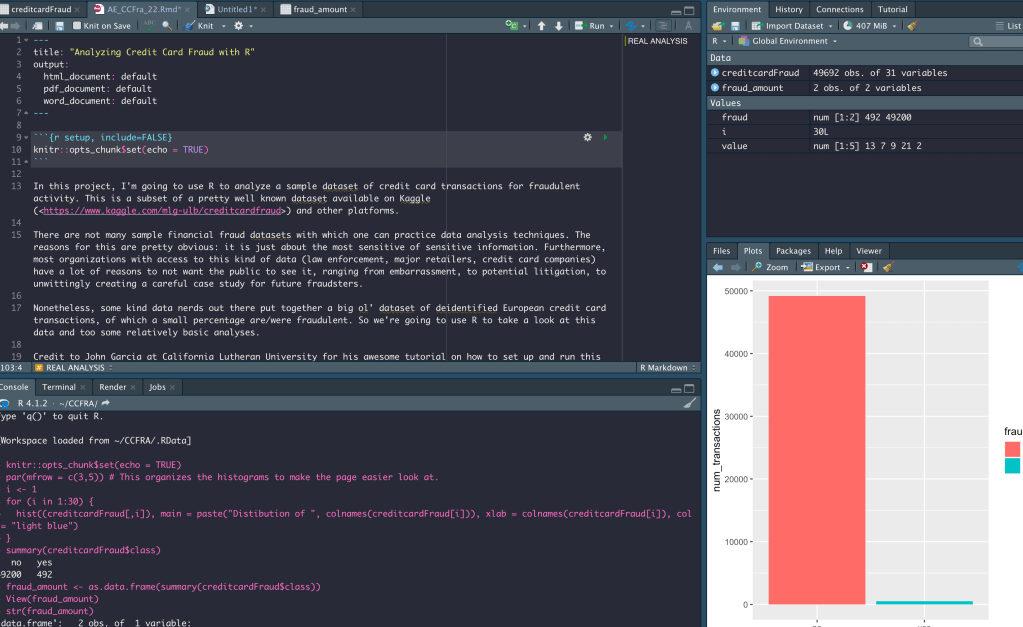
Less than one percent fraudulent. This is pretty consistent with industry estimates. Let’s make a little data frame and viz to check out the sheer difference between these two amounts with some pretty colors.
fraud_amount <- data.frame(fraudulent=c("yes","no"),
                           num_transactions=c(492,49200)) #Call me lazy, but this was easier than converting the summary into its own dataframe with fancy code. I don't care. I like easier over "impressive."

ggplot(data=fraud_amount, aes(x=fraudulent, y=num_transactions, fill=fraudulent)) +
  geom_bar(stat="identity")

Fun fact: I tried to put these values in several other kinds of viz to change things up (treemap, pie chart), but the “yes” section was so damn small you could barely even see it. That kind shows us right off the bat just how few credit card transactions are fraudulent. Forgive me if I don’t share them with you, unless you’d like to see a giant, unbroken rectangle and/or a giant, unbroken circle.
Now let’s make some little histograms out of the frequency of occurrence of each of the data values
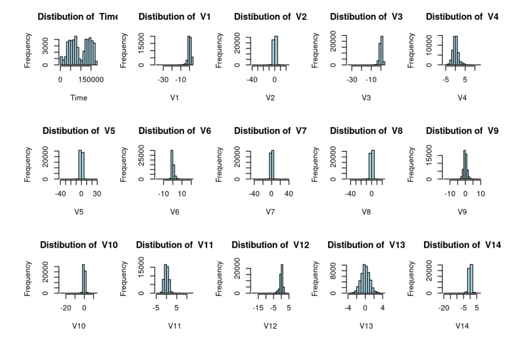

Now we have our nice little histograms that show the frequency of each transaction value in each column, in addition to the somewhat useless total distribution of amounts in the last graph and the distribution of time in the first one. This will set us up for the really wacky and fun stuff we are going to do next. (Again, “wacky” and “fun” are loose terms when it comes to principal component analysis and creating sample sets).
The next parts of the analyses start to get a little dense (as if any of this ISN’T ALREADY dense), so let’s wrap up part one for now.
