After I finished up the last project on DC’s homicides by police work shift and ward, I decided I wanted to use SQL to clean the data a little more, and this time analyze the method used to commit the homicides. 

The three variables possible in this dataset for method are:

• Gun
• Knife
• Others

“Others” can presumably refer to all of the following: blunt force trauma, arson, vehicular homicide, poisoning, asphyxiation, drowning, narcotics, and criminal neglect. It may even refer to other cutting instruments, but I imagine those are probably categorized under “knives” by the MPD. (By the way, I’m not that twisted so as to sit here and think of all of this: The FBI’s Uniform Crime Report actually breaks down common homicide methods in a more detailed way on their website.)

Now, onto the data.

I could grab all the data and get it SQL ready by using Tidyverse tools in R, or analogous ones in Python, but to be honest, there are so few columns here that it won’t be too bad to do it manually. 

Another time. 

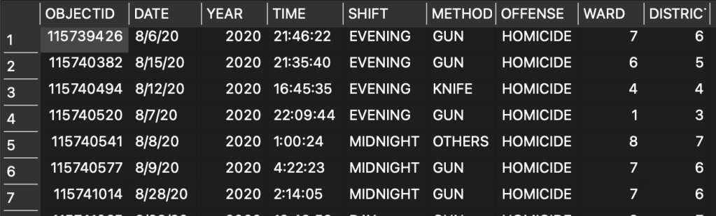
First, I grabbed the Crime Incidents in 2019, 2020, and 2021 .csv files from Open Data DC. Then, I pared down the unnecessary columns and removed the non-homicide rows just like in the previous project. Next, I needed to pick a RDBMS to do my SQL queries with. I decided to use SQLite Studio for simplicity’s sake. It doesn’t have all the capabilities of PostgreSQL or MSSQL Server through Azure Data Studio, but I’m not doing anything too crazy with this data today.

So I open up SQLite and create a new database with the awkward name “dchommeth.” This sounds like some kind of biblical verb, or something perhaps more nefarious. 

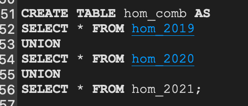
In my experience, it goes a little faster to just write out the command to create a new table, rather than inputting every single variable into the graphical user interface.  For the Homicides in 2021 table, it looked a little something like this:

I just copied this code and repeated it for the other two tables for 2020 and 2021.

Now let’s first take a look at what different types of methods were used in DC’s homicides for 2021. 

So right here we can see that firearm homicides were the most common in 2021. Let’s take a look at other years.

Here’s 2020.

And here’s 2019.

Now I’m going to make a table that combines all the values from all of the tables. I want to do this for two reasons: 1) It makes later queries and analysis a little bit simpler and 2) As I mentioned in my post on the workshift and ward project, I don’t completely trust Open Data DC to have all of their time/data consistent across their .csv files. (Recall that their shift times were totally wrong in the other project.) By combining the three tables together, extracting the years out, and doing SQL queries based on year as a separate variable, we will ensure that we are in fact querying the correct data.

Either way, I’ll call this new combined table the incredibly creative name of hom_comb, or homicides combined. 

It said it affected 583 rows. Let’s make sure this is the right amount. I’m going to make a new table that’s just the counts of the totals of all of the individual tables. I’ll call it hom_tot for homicide total.

And now if we do a sum of these three amounts, we get 583. 

All good!

Now all the values are in one table so they will be much easier to work with. 

Let’s check out the totals by method for all three years, ordered from most to least common:

Wow. Even before breaking down the data even more, we can see the patently absurd disparity between methods of murder in D.C. According to this query, there are almost five times as many murders with guns as all other methods combined.

Now, I want to compare the totals for each method in each year in one single table view. This can get a little tricky, especially in SQLite. First, I’m going to extract just the year out of the date column in the hom_comb table. This will make it easier to run the later aggregate queries, and it will also clear up any D.C.-Open-Data-based disparities in actual-year vs. year-of-table. After some finagling, here is my result, which loaded into a new table called hom_comb_year:

Now, in order to get the totals for each method, I have to take into account that I am essentially the occurrence of string (method) in the table. This is a little bit trickier than just summing up totals in a given column. I could do a complicated COUNT function, but the best option is to use a combination of SUM and CASE WHEN. In so doing, I’ve basically told SQLite to give every occurrence of a particular variable in “method” the value of 1, and to add up those total values and group them by different methods. Here is what that query looks like and the result we get:

So we can already see here that the final totals, after combing through them with SQL queries based on year, are different than the stated totals above. For example, the earlier queries on separate tables (without year being isolated) said there were 70 OTHERS murders. Here, the total is only 67. Upon further review, I see that there were a couple of stragglers from 2017 and 2018 in my 2019 dataset. This might have something to do with the discovery of a body late, or it could just have something to do with a problem in the D.C. Open Data system.

The reality is, this realization makes me question the integrity of some of the other variables in the dataset. In fact, this type of aberration is notoriously common in crime data, and for years even the FBI’s UCR data has been criticized by academics as unreliable. But thank goodness this is just a blog post and not an academic paper being intended to shape policy. This is why it’s always important to clean your data as precisely as possible.

In any event, I’m going to save these values into a new table called hom_tot_year which I will export as a .csv to mess with for visualizations. 

Even if there are some flaws with the data, we can pretty safely say that firearms are the main method – by far – of committing homicides in Washington, D.C. Let’s take a look at the comparisons as a visualization in Tableau. The contrast is stark.

Unsurprisingly, firearm homicides make up the vast majority of murders in D.C. This is pretty consistent with violence in the rest of the country, but still higher. Here’s the FBI’s data on the whole country:

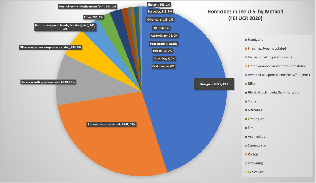
Taking a look at the FBI’s UCR for the year of 2020, we can readily see that the various categories of firearm make up roughly 78% of all murders in the U.S; the other categories of murder weapon pale in comparison.

D.C.’s percentages are similar, but higher for guns, and even more markedly so in 2020:

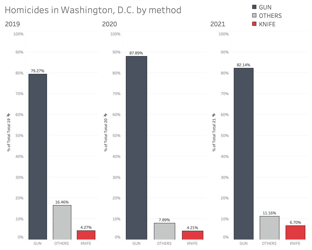
Murders with knives and other cutting instruments are much lower in D.C. than in the rest of the country, but are readily made up by the increase in murders with a firearm. But we have to remember, this is a geographically compact urban area being compared with data from an entire country at large. In that vein, it would be interesting to compare D.C.’s rates of murder weapon usage with other urban areas throughout the United States.

But that’s an investigation for another day.

Either way, the situation is not good, and it remains to be seen what can be done about the spiking murder rate, not only in D.C., but in the rest of the country’s major cities as a whole.